Linear Regression

Additional linear-regression visualizations

Historical Origin: Regression to the Mean

• In the 19th century, Francis Galton studied parent and child heights.

• He observed that extreme values tend to be followed by values closer to the average.

• He called this pattern regression toward mediocrity (now: regression to the mean).

Why this matters:
The term regression originally came from this statistical phenomenon, before modern ML usage.

Francis Galton (via Wikipedia/Wikimedia Commons)

Motivation

Why linear regression matters in practice.

Goal of Regression

• I own a house in King County.

• It has 3 bedrooms, 2 bathrooms, a 10,000 sqft lot, and is 10 km away from Bill Gates’ mansion.

• I need a reliable estimate of what it is worth.

How could I estimate the value?

• Use training data to …

• … find one similar house …

• … and use its value as an estimate.

Use training data to …

… learn a general rule …

… and apply it to estimate value.

I should train a regression model

    216 645  $ base price

+    20 033  $ for each bedroom

+   234 314 $ for each bathroom

+         1 $ for each sqft of lot size

-    14 745 $ for each km distance from Bill Gates' mansion

=        xyz $ estimated house price

Note:
The term regression (e.g. regression analysis) usually refers to linear regression.
(Don't confuse it with logistic regression.)

Building a model

Descriptive statistics

Using linear regression for explanation (profiling)

\(\rightarrow\) Why is my house worth xyz?

\(\rightarrow\) How can I increase the price?

Inferential statistics

Using linear regression for prediction

\(\rightarrow\) How much is my house worth?

Linear Equation

Linear Equation

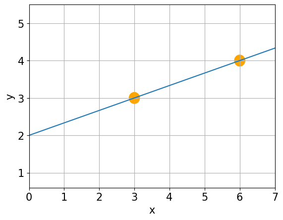
Question: What is the equation of a line?

Linear Equation

Key terms:

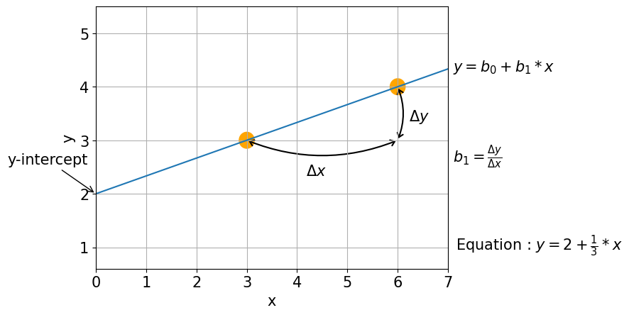
• Intercept (b₀): predicted value of y when x = 0.
• Slope (b₁): expected change in y when x increases by 1 unit.

Linear Regression

Linear Regression

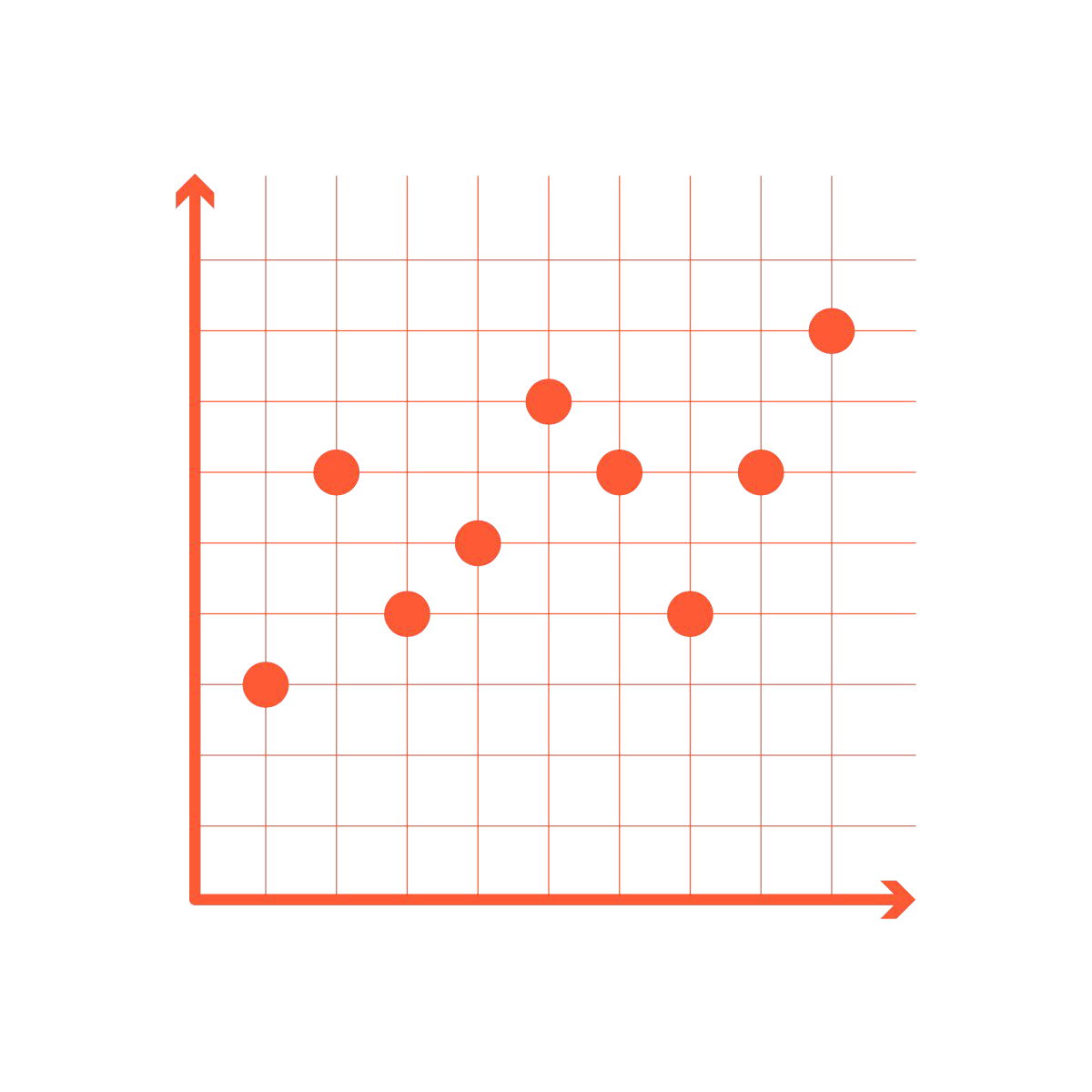
• Is variable \(X\) associated with variable \(y\)?

• If yes, what is the relationship, and can we use it to predict \(y\)?

Note:

• Correlation — measures the strength of a relationship → a number.
• Regression — quantifies the relationship itself → an equation.

What about more than 2 points?

Let’s look at an example

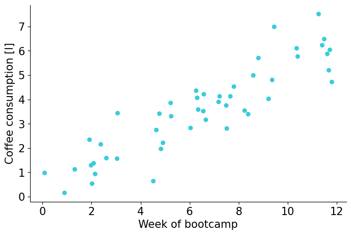
Two correlated variables:

• week of bootcamp, \(x\)

• coffee consumption, \(y\)

• \(r \approx 0.9\)

\(y = b_{0}+b_{1}\cdot x+e\)

\(\rightarrow\) Find \(b_0\) and \(b_1\)

Try two fitted lines. Which one is better?

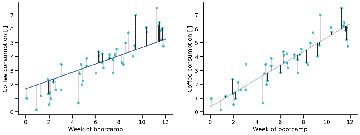
• Grey: \(\hat{y} = 0.35 + 0.5 \cdot x\)

• Blue: \(\hat{y} = 1.65 + 0.3 \cdot x\)

Note:
ŷ ("y-hat") denotes an estimated value (line) rather than an observed value (data point).

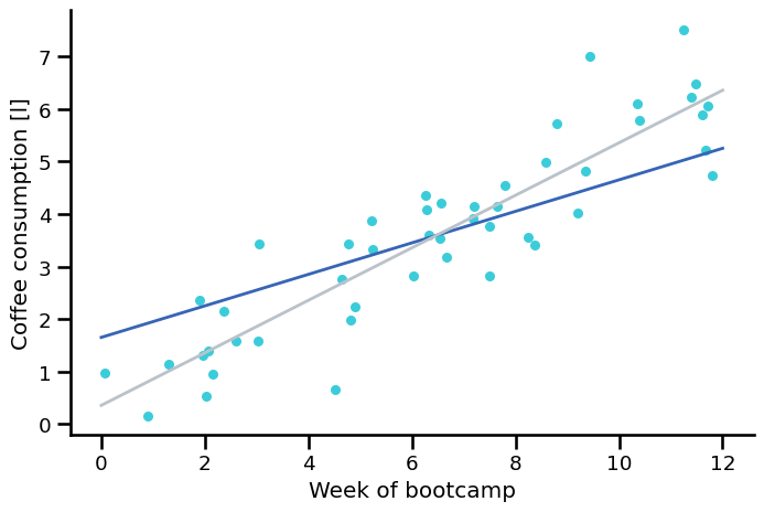
How do we know which line is better?

Residuals

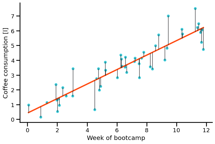
For each observation \(i\):

\[e_i = y_i - \hat{y}_i\]

which means:

\[y_i = b_0 + b_1 \cdot x_i + e_i\]

How to read this:

• Real value (what we observed): \(y_i\)

• Predicted value from the line: \(\hat{y}_i\)

• Prediction error (residual): \(e_i\)

• If the residual is positive (\(e_i\) > 0), we predicted too low; if negative (\(e_i\) < 0), we predicted too high.

Residual Example (One Data Point)

Suppose for one observation:

• Observed value: \(y = 4.8\)

• Model prediction: \(\hat{y} = 0.3 + 0.5 \cdot 6 = 3.3\)

Residual: $\(e = y - \hat{y} = 4.8 - 3.3 = 1.5\)$

Interpretation:

• Positive residual (\(e > 0\)): model underestimates

• Negative residual (\(e < 0\)): model overestimates

Least Squares Criterion

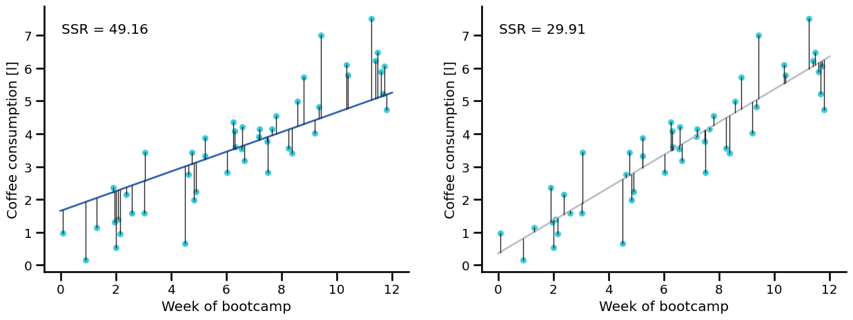
To compare fitted lines, we use the sum of squared residuals:

\[ J(b_{0}, b_{1}) = \sum_{i=1}^{n} e_{i}^{2} = \sum_{i=1}^{n}(y_{i} - \hat{y}_{i})^{2} = \sum_{i=1}^{n}(y_{i} - (b_{0} + b_{1}x_{i}))^{2} \]

\[ n \text{ is the number of observations} \]

How to read this equation:

• Compute error for each point: \(y_i-\hat{y}_i\)

• Square each error (no cancellation, large errors count more)

• Add all squared errors \(\rightarrow\) this total is \(J\)

• Smaller \(J\) means a better-fitting line.

Trying several fitted lines

By comparing the sum of squared residuals, we can decide which line fits better:

\[ J(b_{0}, b_{1}) = \sum_{i=1}^{n} e_{i}^{2} = \sum_{i=1}^{n}(y_{i} - \hat{y}_{i})^{2} = \sum_{i=1}^{n}(y_{i} - (b_{0} + b_{1}x_{i}))^{2} \]

Beginner view:

• Each candidate line gets one score: \(J\)

• Lower score = line stays closer to points overall.

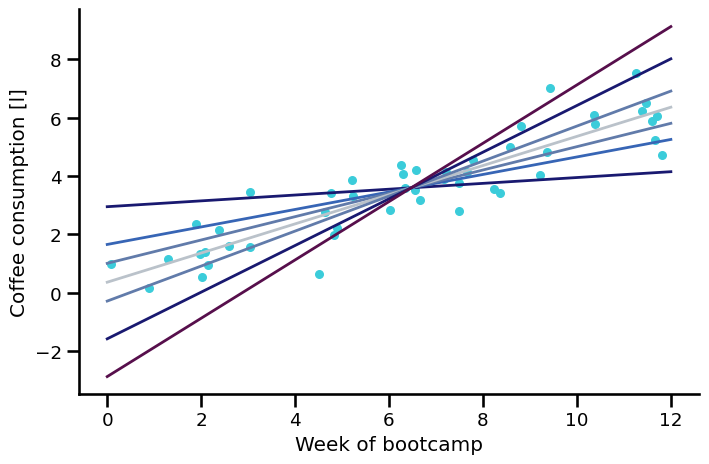
There are infinitely many possible lines

So how do we solve this?

• Doing this manually is not scalable

• We minimize the OLS objective \(J(b_0, b_1)\) with respect to \(b_0\) and \(b_1\)

• OLS = Ordinary Least Squares

\[ J(b_{0}, b_{1}) = \sum (y_{i} - b_{0} - b_{1}x_{i})^{2} \]

Plain language:

• Try values for \(b_0\) (intercept) and \(b_1\) (slope)

• Keep the pair that makes \(J\) as small as possible.

Ordinary Least Squares Regression

\[ \mathrm{min}\ J(b_{0},b_{1})\ =\ \sum(y_{i}\ -\ b_{0}\ -\ b_{1}x_{i})^{2}\]

\[\begin{split}\begin{align} \frac{\partial J}{\partial b_{0}}&=\mathrm{-2\,}\Sigma(y_{i}-b_{0}-b_{1}x_{i})\nonumber\,=\,0 \\ \frac{\partial J}{\partial b_{1}}&=\mathrm{-2\,}\Sigma x_i(y_{i}-b_{0}-b_{1}x_{i})\nonumber\,=\,0 \end{align}\end{split}\]

Divide the first equation by \(2n\):

\[\begin{split} \begin{array}{c}{{-(\bar{y}\ -\ b_{0}\ -\ b_{1}\bar{x})\ =\ 0}} \\ {{b_{0}\ =\ \bar{y}\ -\ b_{1}\bar{x}}}\end{array}\end{split}\]

… more algebra gives:

\[ b_1 = \frac{\Sigma(y_i - \bar{y})(x_i - \bar{x})}{\sum(x_{i} - \bar{x})^{2}} \]

How to interpret:

• ∂J/∂b_j means how much J changes when one parameter changes.
• Setting derivatives to 0 gives the minimum for this problem.
• Result: formulas for the best b₀ and b₁.

Useful facts about residuals

\[\begin{split}\begin{align} y_i &= b_0 + b_1 \cdot x_i + e_i \\ e_i &= y_i -b_0 -b_1 \cdot x_i \\ b_0 &= \bar{y} - b_1 \cdot \bar{x} \end{align}\end{split}\]

Which leads to the following conclusions:

\[\begin{split}\begin{align} \Sigma e_i &= 0 \\ \Sigma(x_i - \bar{x}) \cdot e_i &= 0 \end{align}\end{split}\]

Note:

• The second equation means residuals are uncorrelated with the explanatory variable.
• Feel free to verify this on your own fitted models.

Model performance

Mean of target variable: \(\bar{y}=\frac{1}{n} \sum\limits_{i=1}^{n}y_{i}\)

Variance of target variable: \(\sigma^2 = \frac{1}{n-1}\sum_i{(y_i-\bar{y})^2}\)

How to read:

• Mean: add all target values and divide by how many values there are.

• Variance: average squared distance from the mean (how spread out values are).

Baseline Mean vs Fitted Regression

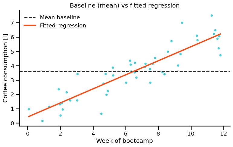
A constant mean line is a simple baseline model. A fitted regression line should reduce error compared with this baseline.

Sum of Squares Decomposition (Variance Analysis)

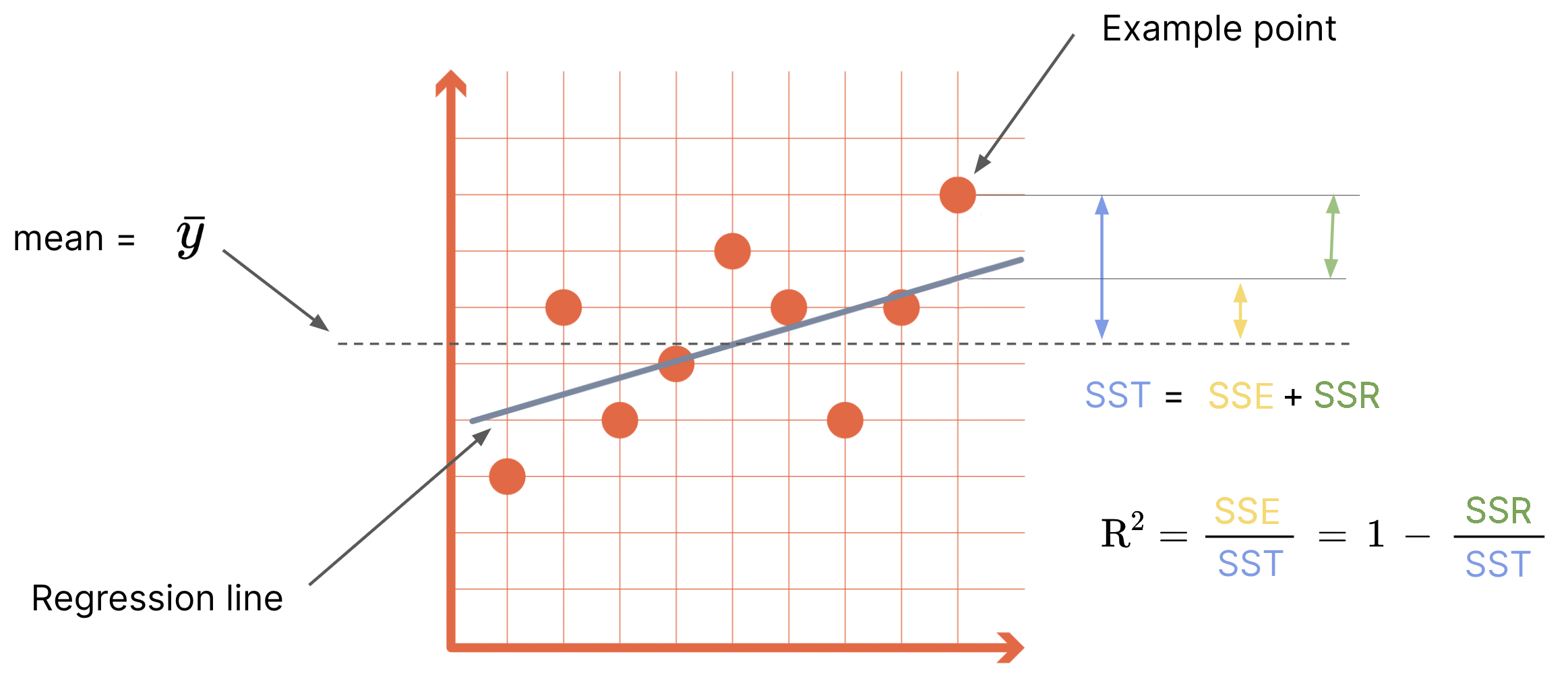
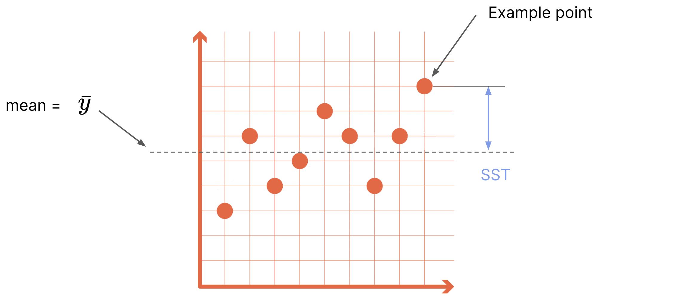
SST = total sum of squares
SSE = explained sum of squares
SSR = residual (unexplained) sum of squares

\[SST = SSE + SSR\]

Note: These quantities are scale-dependent, so their absolute values depend on the scale of y.
0 ≤ R² ≤ 1
R² = SSE / SST = 1 - SSR / SST
Interpretation: higher R² means the model explains more of the target variability.

Root Mean Squared Error

\[ RMSE = \sqrt{\frac{1}{n}\sum_{i=1}^{n}\left(y_{i}-{\hat{y}}_{i}\right)^{2}} \]

How to compute RMSE:

1. Compute each residual \((y_i-\hat{y}_i)\)

2. Square residuals

3. Average them \(\rightarrow\) MSE

4. Take square root \(\rightarrow\) RMSE

Note:
RMSE is in the same unit as y (easy to interpret).
Lower RMSE means better predictions on average.

Which Metric Answers Which Question?

• RMSE: “How large is the typical prediction error?” Units: same as target variable \(y\)

• \(R^2\): “How much variance does the model explain?” Range: 0 to 1 (higher is better)

• Adjusted \(R^2\): “Did extra features truly help?” Penalizes adding weak or unnecessary features

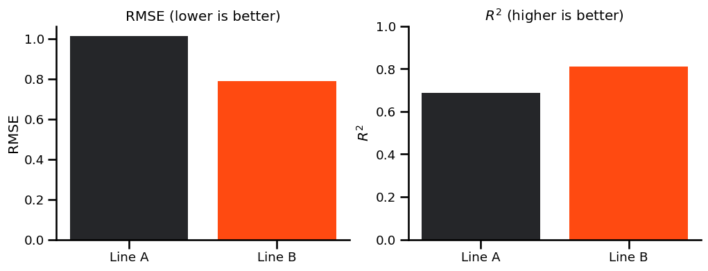
Metric Comparison for Two Candidate Lines

Same dataset, two fitted lines. Use RMSE and \(R^2\) to compare their quality directly.

Key Terms

Key terms: Machine learning

Variables:

• Target (dependent variable, prediction, response, y)

• Feature (independent variable, explanatory/predictive variable, attribute, X)

• Observation (row, instance, example, data point)

Model:

• Fitted values (predicted values) - denoted with the hat notation \(\hat{y}\)

• Residuals (errors, e) - difference between reality and model

• Least squares (method for fitting a regression)

• Coefficients, weights (here: slope, intercept)

But I want to use more than one feature

Multiple Linear Regression

Multiple regression

For one feature: \(y=b_0+b_1x+e\). For many features: \(y=Xb+e\).

Where y, b, e are vectors, and X is a matrix.

\[\begin{split} y = \begin{bmatrix} y_1 \\ \vdots \\ y_n \end{bmatrix}, \quad X = \begin{bmatrix} 1 & x_{11} & \cdots & x_{1m} \\ \vdots & \vdots & \ddots & \vdots \\ 1 & x_{n1} & \cdots & x_{nm} \end{bmatrix} \end{split}\]

\[\begin{split} b = \begin{bmatrix} b_0 \\ b_1 \\ \vdots \\ b_m \end{bmatrix}, \quad e = \begin{bmatrix} e_1 \\ \vdots \\ e_n \end{bmatrix} \end{split}\]

\(n\) = number of observations, \(m\) = number of features.

\(x_{obs,feature} = x_{row,col} = x_{n,m}\)

\(y\) and \(X\) are known (observed data). \(b\) and \(e\) are unknown.

Think of \(Xb\) as: for each row, multiply features by weights and add them up.

Note:
Multiple regression means multiple independent variables. Multivariate regression means multiple dependent variables.

Normal Equation

The optimal values for \(b\) (\(b_0\), \(b_1\), \(...\), \(b_m\)) are often found numerically (e.g., gradient descent). For linear regression, they can also be computed analytically with the normal equation:

(1)\[b = (X^TX)^{-1}X^Ty\]

Predictions

Once \(b\) is known, we can make predictions: $\( \hat{y} = b_0 + b_1x_1 + ... + b_mx_m \)$

Or in matrix notation:

\[\hat{y} = Xb\]

\(X\) needs the same feature format as above, but can have a different number of rows (e.g., 1). The error term \(e\) remains unknown, but is minimized during fitting.

Multiple Regression — Evaluation Metrics

Root Mean Squared Error (RMSE)

\[ RMSE = \sqrt{\frac{1}{n}\sum_{i=1}^{n}\left(y_{i}-{\hat{y}}_{i}\right)^{2}} \]

  Typical prediction error size in the original unit of \(y\).
  Lower RMSE is better.

Adjusted R-squared (\(adj.\ R^2\)):

\[ adj.\;R^{2}=1-\left(1-R^{2}\right)\frac{n-1}{n-p-1}\]

  \(n\): sample size, \(p\): number of features.
  Starts from \(R^2\), then penalizes unnecessary features.

Note: Use RMSE for error magnitude and adjusted R² to check if extra features are truly useful.

Overview of Linear Regression Terms

• \(R\): Pearson correlation coefficient — in the interval [-1, 1]

• \(R^2\): Coefficient of determination — fraction of variance in \(y\) explained by the model

• \(MSE\): mean squared error — average squared prediction error

• \(RMSE\): root mean squared error — square root of MSE in the original unit of \(y\)

• \(SST\), \(SSE\), \(SSR\): sum of squares — total, explained, residual

• \(\sigma^2\): variance of a variable — dispersion around the mean

Beginner shortcut:

• Residuals tell you point-by-point errors.
• RMSE tells you average error size.
• R² tells you how much variance your model explains.

References

There are also many detailed explanations in the exercise repositories.

Practical Statistics for Data Science - Peter Bruce & Andrew Bruce

Econometric Methods with Applications in Business and Economics - Christiaan Heij, Paul de Boer, Philip Hans Franses, Teun Kloek, Herman K. van Dijk

Written explanation of LR

Difference between \(R^2\) and adjusted \(R^2\)

StatQuest: Linear Regression

Some more math for those who want to know how to calculate \(b_1\)

\(-2 \Sigma x_i(y_i - b_0 - b_1x_i) = 0 \)

we know that \(b_0 = \bar{y} - b_1 \bar{x}\)

\(-2 \Sigma x_i(y_i - \bar{y} + b_1 \bar{x} - b_1x_i) = 0 \)

\(\Sigma(x_iy_i - x_i \bar{y} + b_1(x_i \bar{x} - x_ix_i)) = 0\)

\(\Sigma(x_iy_i - 2x_i \bar{y} + \bar{x}\bar{y} + b_1(-\bar{x}\bar{x} + 2x_i \bar{x} - x_ix_i)) = 0 \hspace{1cm}|\hspace{1cm} \Sigma x_i = \Sigma \bar{x} \)

\(\Sigma(x_iy_i - x_i \bar{y} - \bar{x}y_i + \bar{x}\bar{y} + b_1(-\bar{x}\bar{x} + 2x_i \bar{x} - x_ix_i)) = 0 \hspace{1cm}|\hspace{1cm} \Sigma x_i \bar{y}= \Sigma \bar{x}y_i = n \bar{x}\bar{y} \)

\(\Sigma(y_i - \bar{y})(x_i - \bar{x}) - b_1 \Sigma(x_i - \bar{x})^2 = 0 \)

\(b_1 = \frac{\Sigma(y_i - \bar{y})(x_i - \bar{x})}{\Sigma(x_i - \bar{x})^2} \)