Regularization

Part 1

Recap on Bias-Variance Trade-Off

Bias - Variance Trade-Off

\[MSE(\hat{y})=Bias^{2}+Variance+Noise\]

→ to minimize the cost we need to find a good balance between the Bias and Variance term of a model
→ we can influence bias and variance by changing the complexity of our model

Note: Noise is the irreducible error of a model. We cannot influence it.

Example: Underfitting vs. Overfitting

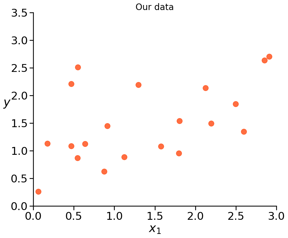
• We got data. But we don’t know the underlying Data Generating Process.

• So we want to model it.

• Do you see a pattern/trend?

Example: Underfitting vs. Overfitting

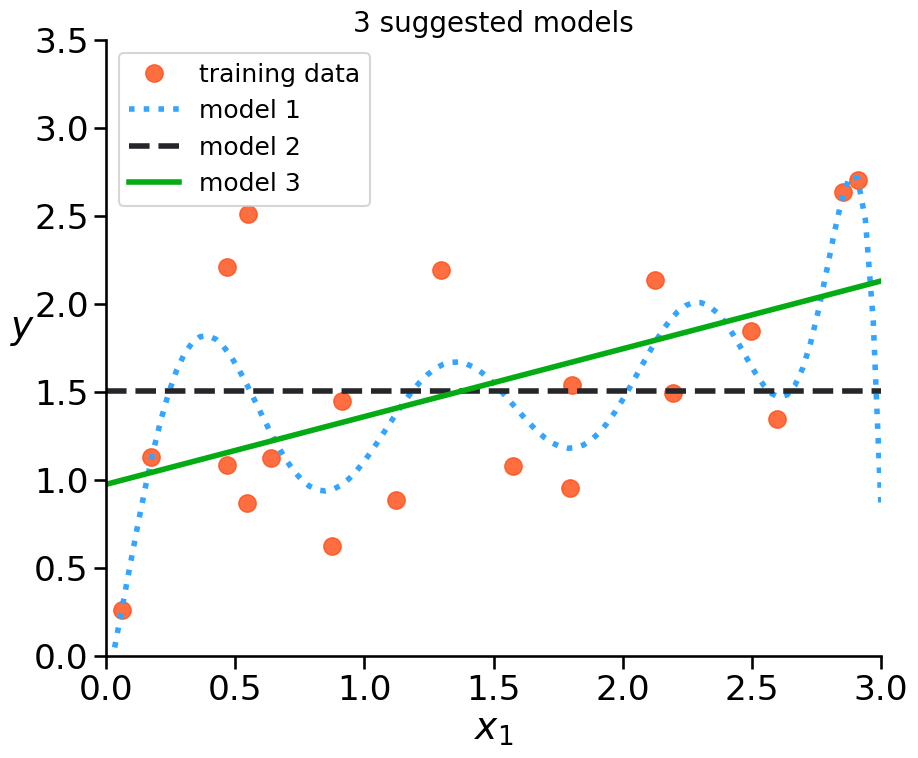
• Which model seems best?

• Which model seems to underfit the data?

• Which model might overfit the data?

• How to evaluate if a model is underfitting/overfitting?

Example: Underfitting vs. Overfitting

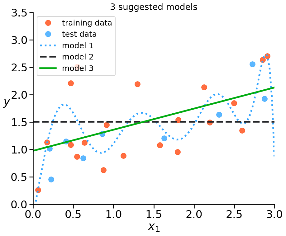
How to evaluate if a model is underfitting/overfitting?

• we need a cost function

• we need test data

• we should do error analysis

Example: Underfitting vs. Overfitting

How to figure out if your model is overfitting?

Example: Underfitting vs. Overfitting

How to figure out if your model is overfitting?

• error on training data is low

• error on test data is high

→ model memorizes the noise in the data

Example: Underfitting vs. Overfitting

How to figure out if your model is overfitting?

• error on training data is low

• error on test data is high

Part 2

A Visual Approach

Prevent Overfitting

If we see overfitting of our model, we could gather more data.

Prevent Overfitting

If we see overfitting of our model, we could reduce its complexity.

HOW?

Note: Every model type has a way to reduce model complexity.
We just learnt Linear Reg. that’s why we will concentrate on the Regularization of those models for now.

Prevent Overfitting

If we see overfitting of our model, we could reduce its complexity.

HOW?

• reduce amount of features

Prevent Overfitting

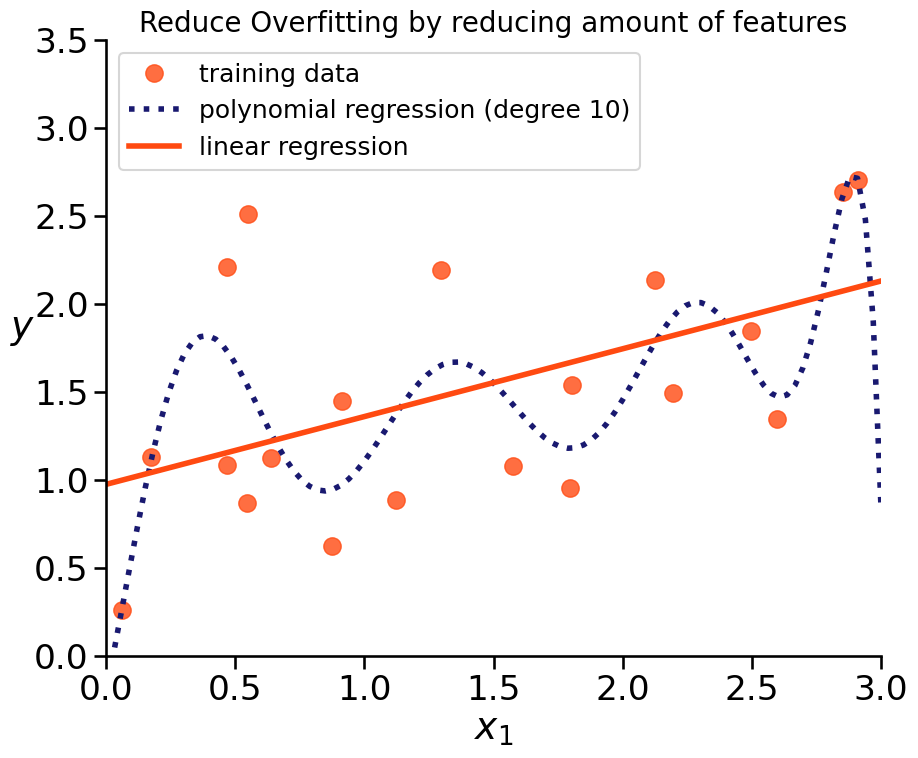
If we see overfitting of our model, we could reduce its complexity.

HOW?

• reduce amount of features

• make the model less susceptible to data by reducing the influence of features
  → smaller coefficients

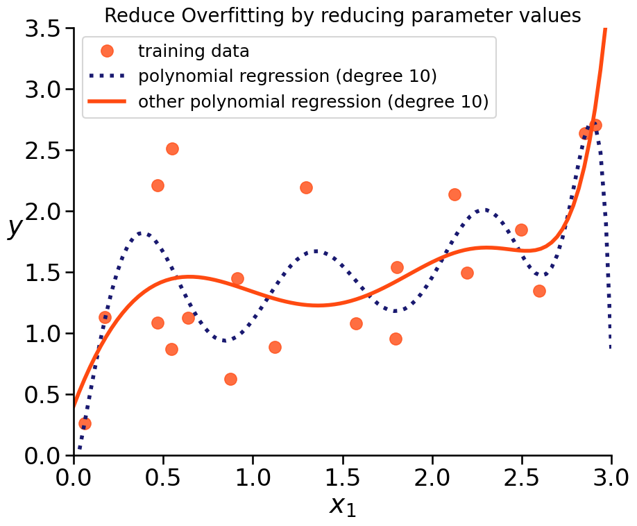
Prevent Overfitting with Regularization

BOTH can be achieved with regularizing a model:

• reduce amount of features

• make the model less susceptive of data by reducing the influence of features (smaller coefficients)

Part 3

Regularization

Regularization

Regularization conceptually uses a hard constraint to prevent coefficients from getting too large, at a small cost in overall accuracy. With the aim to get models that generalize better on new data.

Note: Even with linear models, it can be useful to regularise them. Because they have a tendency to trace outliers in the training data.

Hard constraint

We add a hard constraint to our cost function:

\[\mathrm{min}\,J(b_{0},b_{1})={\frac{1}{n}}\sum{(y_{i}-b_{0}-b_{1}x_{i})}^{2}\,\text{subject}\,\text{to}\,-1 \leq b_{1} \leq 1\]

General form of the constraint:

\[-t \leq b_{1} \leq t\]

What do we have to change to get to a form like this:

\[b_{1} \leq t\]

Note: We are not constraining the y-intercept

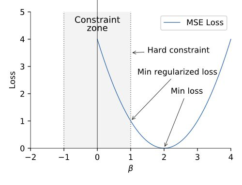
Hard constraint

We add a hard constraint to our cost function:

\[\mathrm{min}\,J(b_{0},b_{1},...,b_{m})={\frac{1}{n}}\sum{(y_{i}-b_{0}-b_{1}x_{i}-...-b_{m}x_{m})}^{2}\,\text{subject}\,\text{to}\,L1/L2\,\text{constraint}\]

The most common regularization constraints:

\[\begin{split}\begin{align} L_{1}\,&:\,|b_{1}| \leq t \\ L_{2}\,&:\,b_{1}^2 \leq t \end{align}\end{split}\]

Hard constraint with more features

We add a hard constraint to our cost function:

\[\mathrm{min}\,J(b_{0},b_{1},...,b_{m})=\frac{1}{n}\sum{(y_{i}-b_{0}-b_{1}x_{i}-...-b_{m}x_{m})}^{2}\,\text{subject}\,\text{to}\,L1/L2\,\text{constraint}\]

The most common regularization constraints:

\[\begin{split}\begin{align} L_{1}\,&:\,|b_{1}|+|b_{2}|+... \leq t \\ L_{2}\,&:\,b_{1}^2+b_{2}^2+... \leq t \end{align}\end{split}\]

Note: If we have more than one feature, we need to bring them all to the same scale. Otherwise they contribute different to the penalty term.

Soft constraint

We can add this constraint directly to our Loss function (t becomes alpha (or lambda))

\[\begin{split}\begin{align} Ridge (L2): J(b)&=\frac{1}{n}\sum{\big(y-(b_{0}+b_{1}x_{1}+b_{2}x_{2})\big)}^{2} + \alpha\,(b_{1}^2+b_{2}^2) \\ Lasso (L1): J(b)&=\frac{1}{n}\sum{\big(y-(b_{0}+b_{1}x_{1}+b_{2}x_{2})\big)}^{2} + \alpha\,(|b_{1}|+|b_{2}|) \end{align}\end{split}\]

Alpha is a hyperparameter. Before training the model we need to set it.

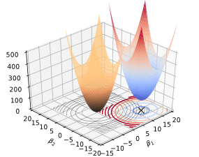
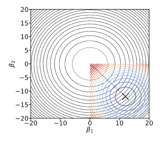
Soft constraint

We can add this constraint directly to our Loss function (t becomes alpha (or lambda))

\[\begin{split}\begin{align} Ridge (L2): J(b)&=\frac{1}{n}\sum{\big(y-(b_{0}+b_{1}x_{1}+b_{2}x_{2})\big)}^{2} + \alpha\,(b_{1}^2+b_{2}^2) \\ Lasso (L1): J(b)&=\frac{1}{n}\sum{\big(y-(b_{0}+b_{1}x_{1}+b_{2}x_{2})\big)}^{2} + \alpha\,(|b_{1}|+|b_{2}|) \end{align}\end{split}\]

What happens if we set alpha to 0?
What happens if we set alpha to a very high value?

Sklearn code for regularization

check sklearn documentation here

ridge_mod = Ridge(alpha=1.0)  #adjust the alpha level
ridge_mod.fit(X, y)
ridge_mod.predict(X)

Some different alpha values

We have to test some values for alpha and check which give us best results on unseen data

print(f'the MSE for Ridge regularization and alpha = 0.5 is:', get_mse(Ridge,X,y, polynomial=True, alpha=0.5))
print(f'the MSE for Lasso regularization and alpha = 0.5 is: ',get_mse(Lasso,X,y, polynomial=True, alpha=0.5))

the MSE for Ridge regularization and alpha = 0.5 is: 0.2957168909631701
the MSE for Lasso regularization and alpha = 0.5 is:  0.4647391677603675

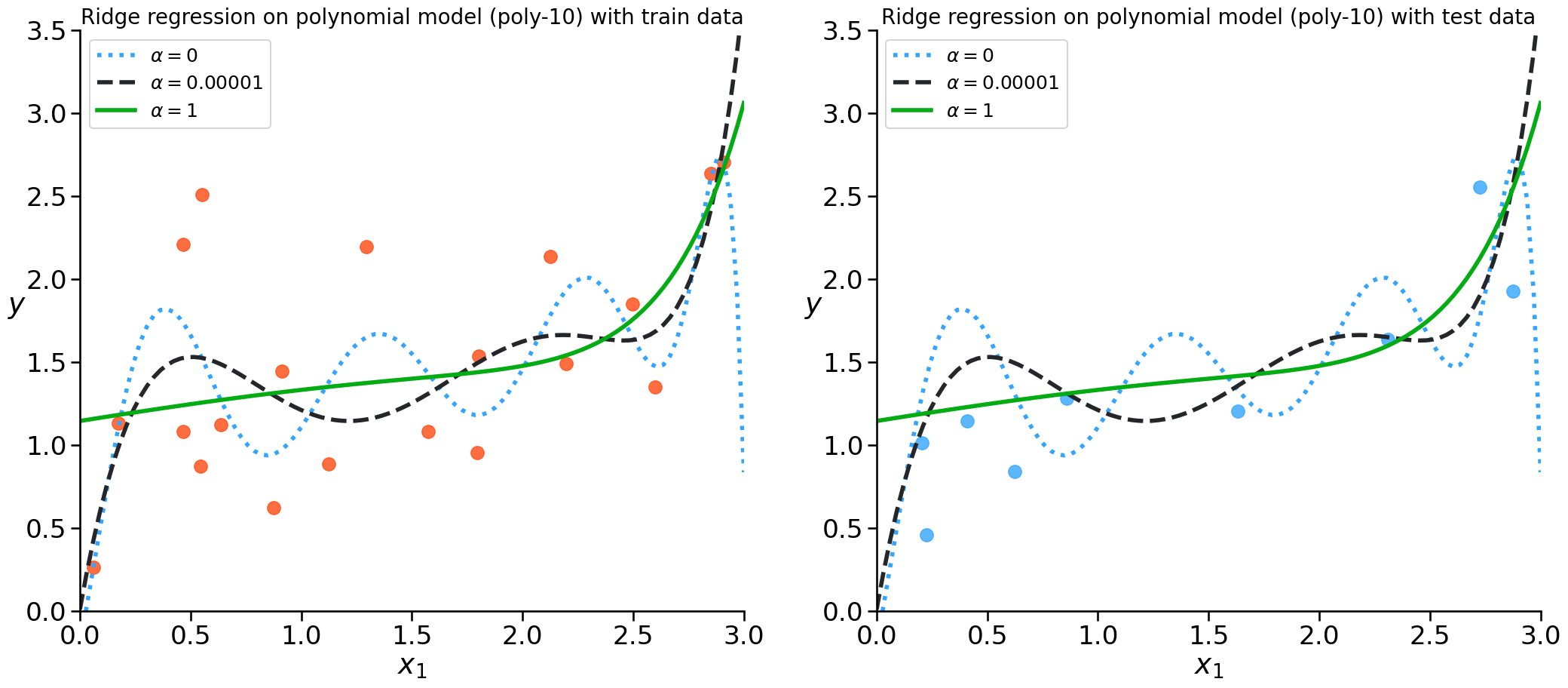
Ridge Regression

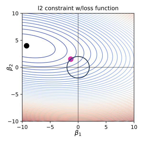
• Also called L2 Regularization / l2 norm

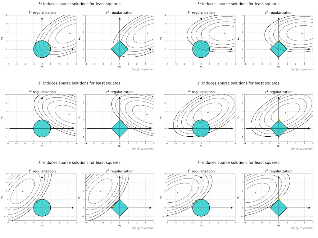
• the regularization term forces the parameter estimates to be as small as possible - weight decay

\[J(b)=\frac{1}{n} \sum{(y-\hat{y}(b))^2}+\alpha\sum{b_{i}^2}\]

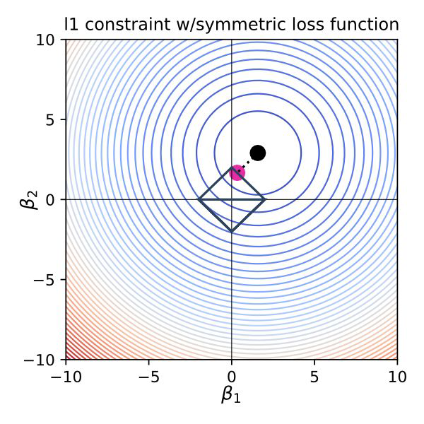
Lasso Regression

Least Absolute Shrinkage and Selection Operator

• Also called L1 Regression / l1 norm

• Tends to eliminate weights = it automatically performs feature selection

\[J(b)=\frac{1}{n} \sum{(y-\hat{y}(b))^2}+\alpha\sum{|b_{i}|}\]

Ridge vs Lasso

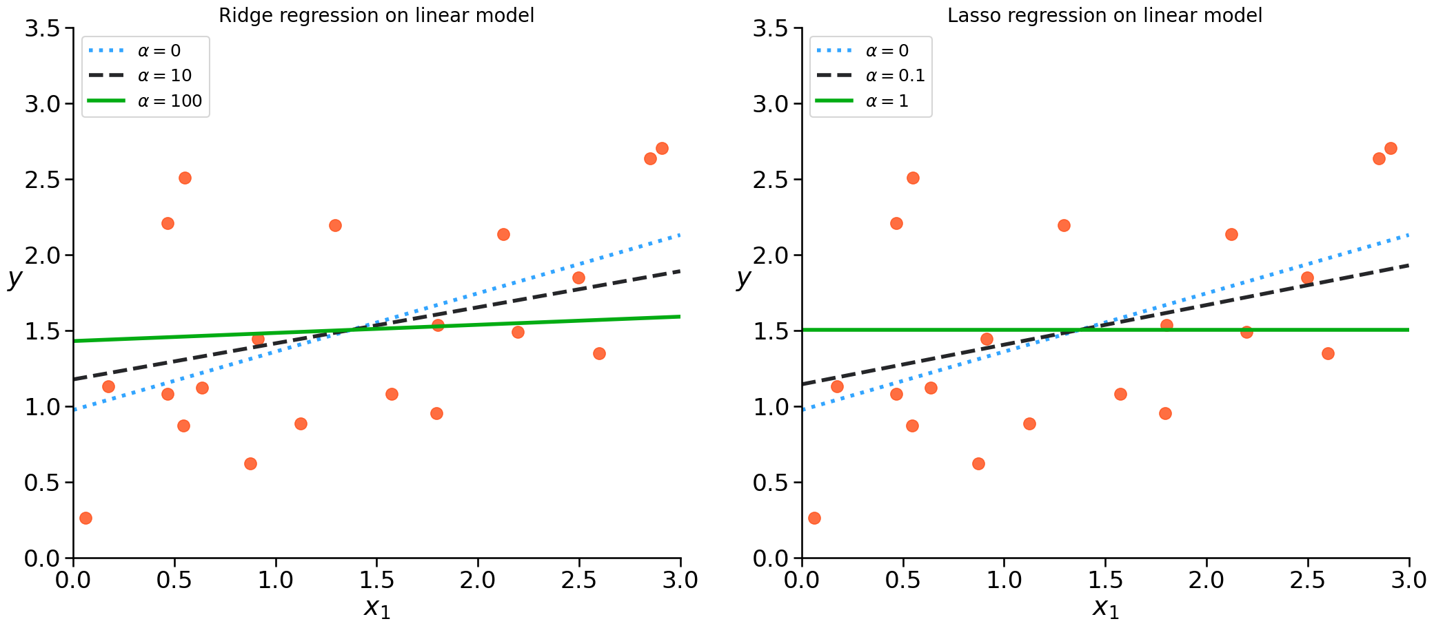
Why is L1 eliminating while L2 only reducing weights?

Elastic Net - Mixing Lasso and Ridge

• Regularization term is weighted average of Ridge and Lasso Regularization term

• When r = 0 it is equivalent to Ridge, if r = 1 it is equivalent to Lasso Regression

• Preferable to Lasso when features are highly correlated or to Ridge for high-dimensional data (more features than observations)

\[J(b)=\frac{1}{n}\sum{(y-\hat{y}(b))}^{2}+\alpha\,r \sum{|b_{i}|+\alpha\,(1-r)} \sum{b_{i}^2}\]

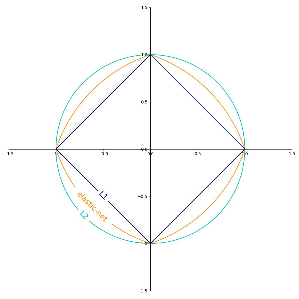
Comparison of regularization methods

• elastic net is between L1 and L2 (whatever you use as r… it will change its form more to L2 or L1

References

• Hands-on ML with scikit-learn and TensorFlow, Geron

• http://scott.fortmann-roe.com/docs/BiasVariance.html

• https://medium.com/analytics-vidhya/bias-variance-tradeoff-for-dummies-9f13147ab7d0

• Machine Learning - A probabilistic Perspective - Kevin P. Murphy

• https://explained.ai/regularization/constraints.html

• https://explained.ai/statspeak/index.html

• https://people.eecs.berkeley.edu/~jrs/189s21/