Gradient Descent#
Orientation#
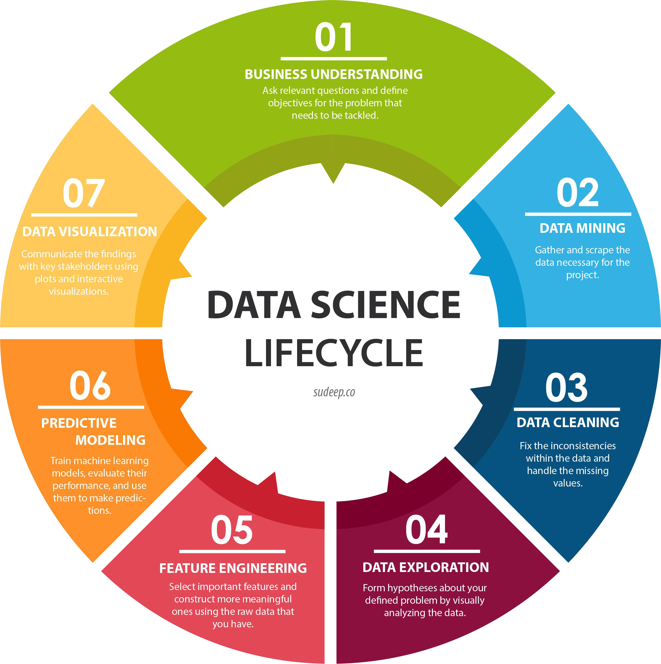
Where is Gradient Descent used in the Data Science Lifecycle?
06 PREDICTIVE MODELING:
select a ML algorithm
train the ML model
evaluate the performance
make predictions
Recap of Optimization of Linear Regression with OLS#
Model: \(y=b_{0}+b_{1}\cdot x+e\)
Residuals: \(e_{i}=y_{i}-\hat{y}_{i}\)
OLS:
Minimize the sum of squared residuals
\(\sum_{i=1}^{n}e_{i}^{2}\)
results in Normal Equation:
\(b=\left(X^{T}X\right)^{-1}X^{T}y\)
→ closed form solution
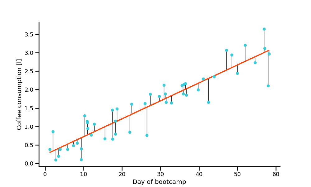
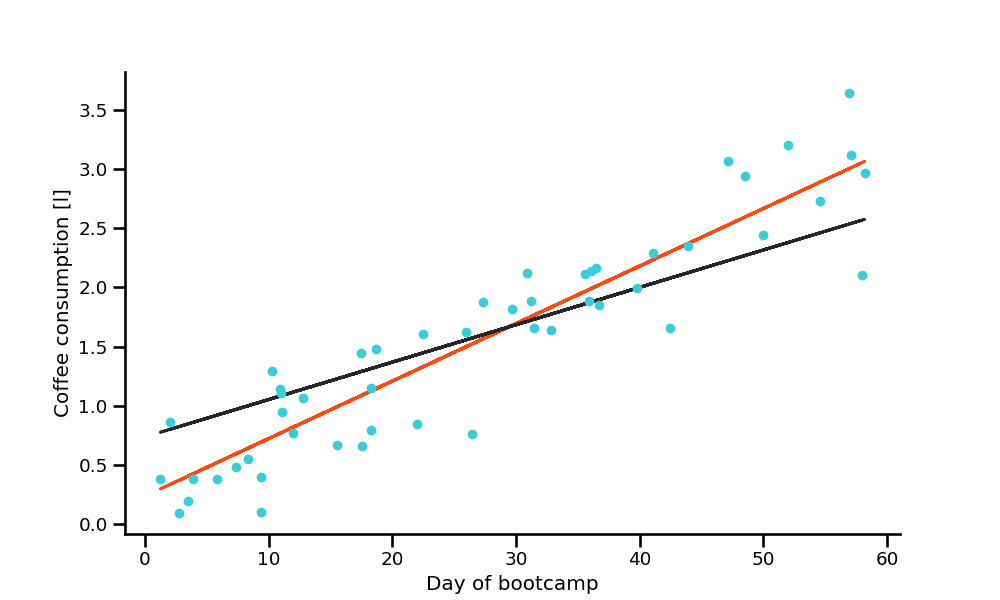
Using OLS (normal equation), the best parameters were found at:
            b₀ = 0.237
            b₁ = 0.049
Definition#
Gradient Descent is an iterative optimization algorithm to find the minimum of a function.
→ e.g. of a cost function

Find the parameters of a model by gradually minimizing your cost#
Go downhill in the direction of the steepest slope.
→ endpoint is dependent on the initial starting point
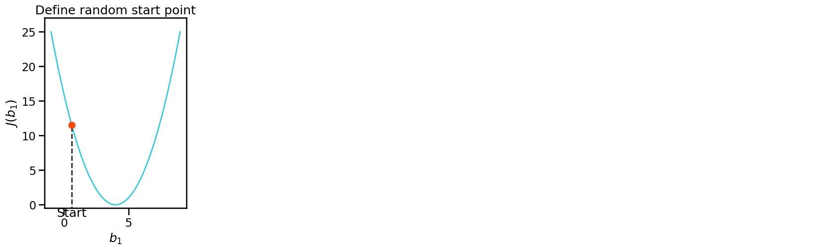
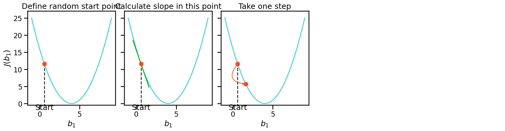
Gradient Descent in a nutshell#
Have some function \(J(b)\)
Want min \(J(b)\):
start with some random parameter \(b\)
keep changing \(b\) to reduce \(J(b)\) until we hopefully get to a minimum
When to use Gradient Descent?#
GD is a simple optimization procedure that can be used for many machine learning algorithms (eg. linear regression, logistic regression, SVM)
used for “Backpropagation” in Neural Nets (variations of GD)
can be used for online learning (update as soon as new data comes in)
gives faster results for problems with many features (computationally simpler)
First Step: Define Model#
Example:
least squares with one feature
Second Step: Define Cost Function#
Mean Squared Error with a little bit of cosmetics (2 in denominator)
\(\hspace{0.5cm}\)
Third Step: Initialize Gradient Descent#
Deliberately set random starting values for \(b\)
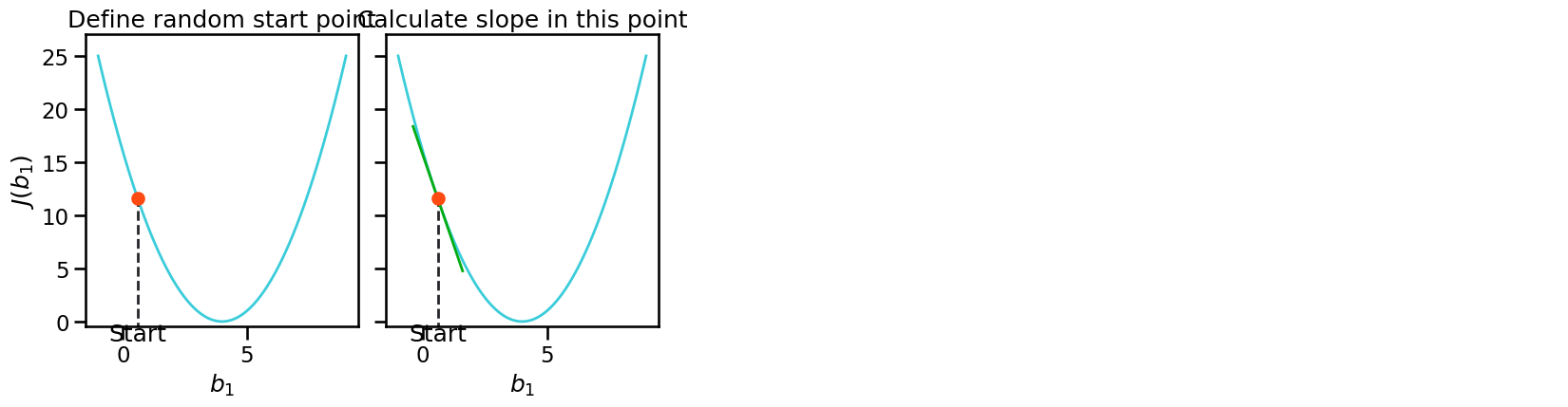
Forth Step: Derivatives with respect to the parameters#
The chain rule gives us:
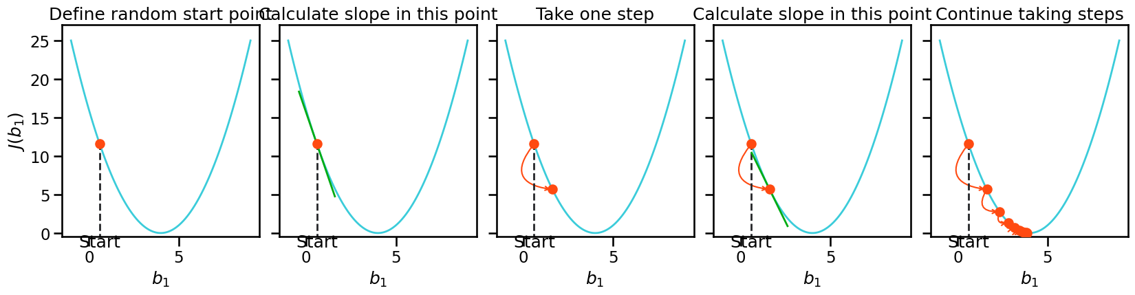
Forth Step: Gradient Descent#
Start descent:
Take derivatives with respect to your parameters \(b\)
Set your learning rate (step-size)
Adjust your parameters (step)
Forth Step: Gradient Descent#
Start descent:
Take derivatives with respect to your parameters \(b\)
Set your learning rate (step-size)
Adjust your parameters (step)
Forth Step: Gradient Descent#
Start descent:
Take derivatives with respect to parameters \(b\)
Set your learning rate (step-size)
Adjust your parameters (step)
Forth Step: Gradient Descent#
Start descent:
Take derivatives with respect to your parameters \(b\)
Set your learning rate (step-size)
Adjust your parameters (step)
Repeat till there is no further improvement
Gradient Descent summed up#
\(\hspace{0.5cm}\)
Define model
Define the cost function
Deliberately set some starting values
Start descent:
Take derivatives with respect to parameters
Set your learning rate (step-size)
Adjust your parameters (step)
Repeat 4. till there is no further improvement

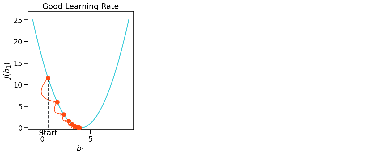
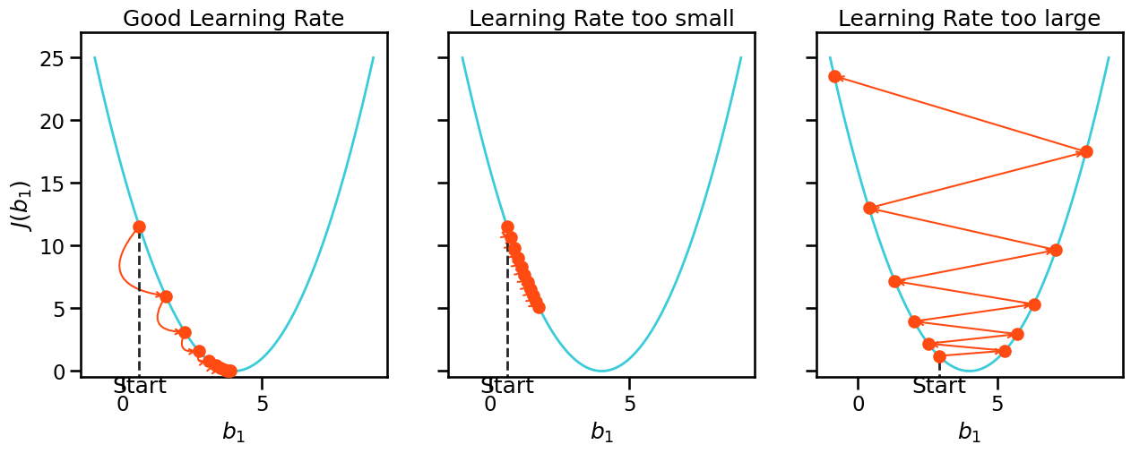
Learning Rate#
It is important to find a good value for the learning rate!
Learning Rate#
It is important to find a good value for the learning rate!
Learning Rate too small → will take long to find optimum
Learning Rate too large → not able to find optimum
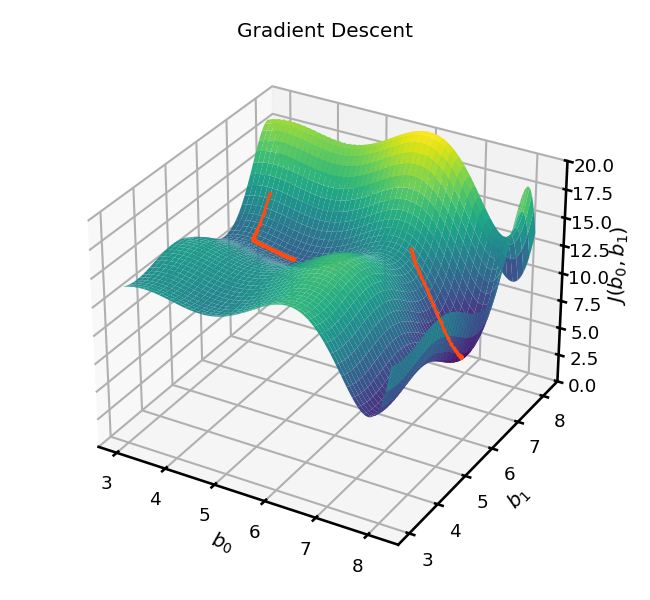
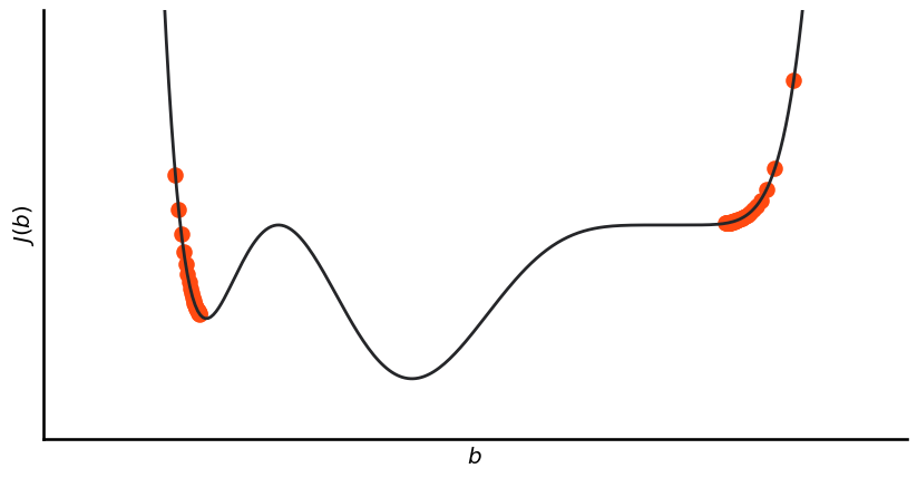
Two main challenges of Gradient Descent#
The MSE cost function for linear regression is a convex function, it just has one global minimum. This is not always the case. Problems are:
local minima
plateaus
Convex: If you pick two random points the line that is connecting them will not cross the curve.
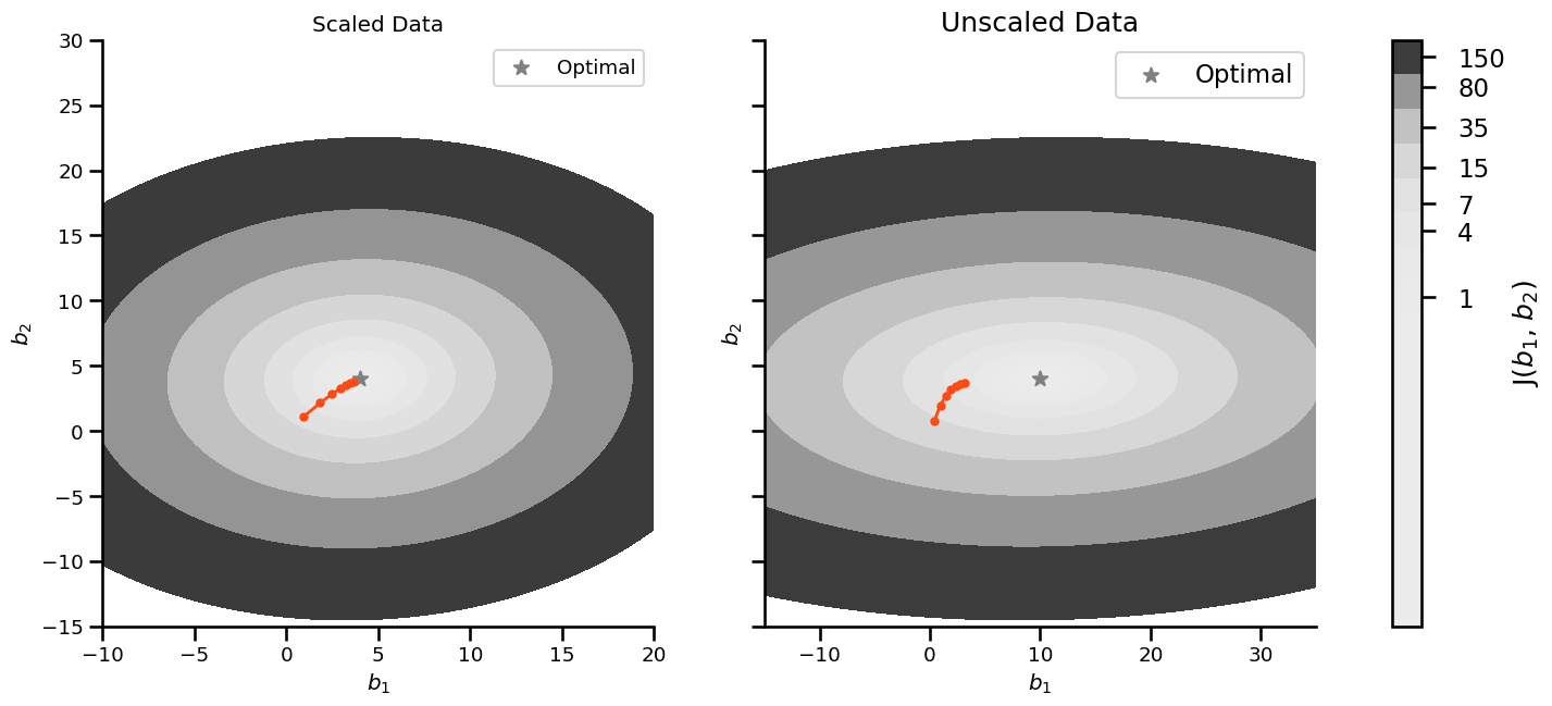
Unscaled Data#
Without scaling the algorithm Gradient Descent needs more time to find the minimum
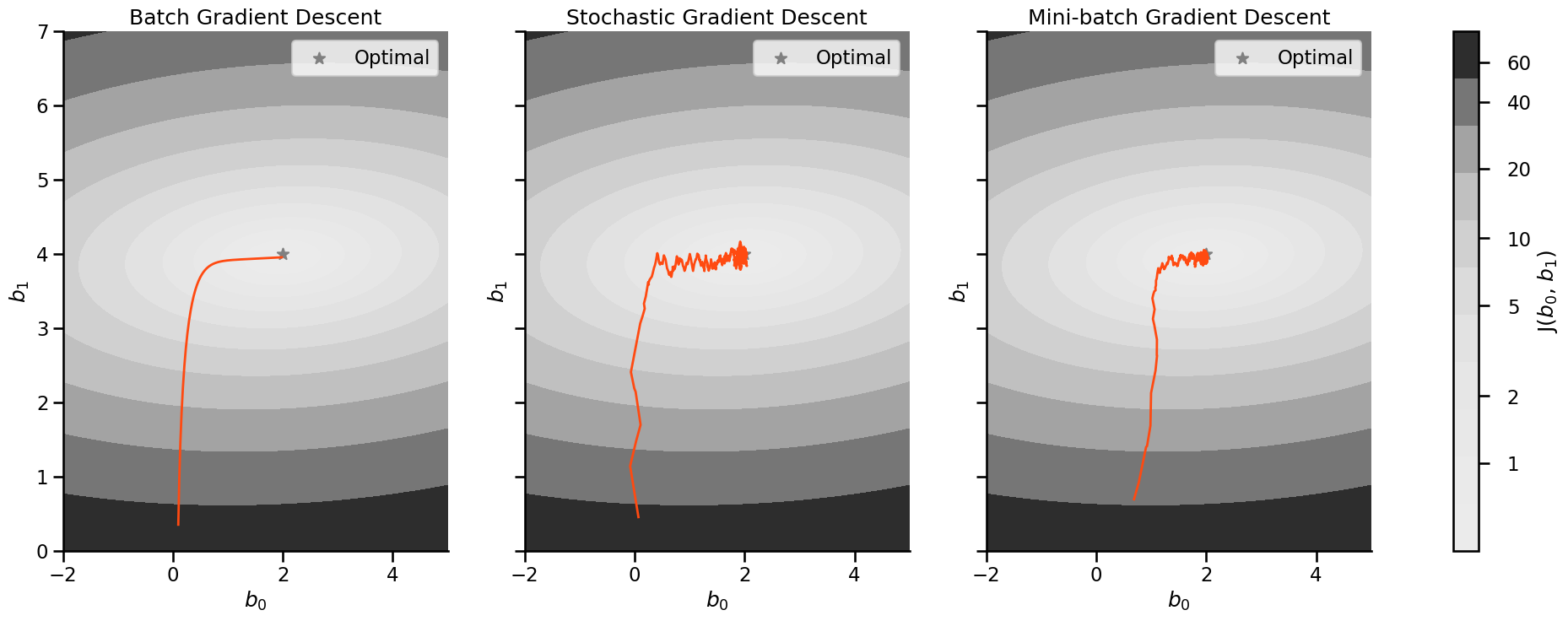
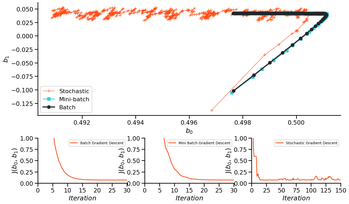
Variants of Gradient Descent#
Which route to take downhill?
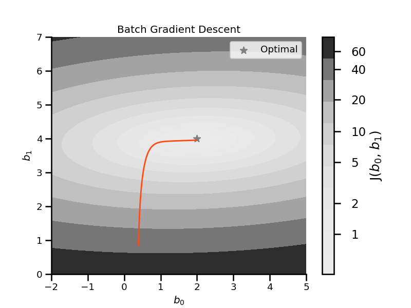
Batch gradient descent#
All instances are used to calculate the gradient (step).
The algorithm is faster than the Normal Equation but still slow.
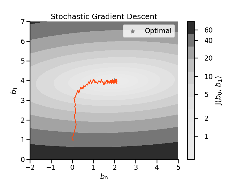
Stochastic gradient descent#
Only 1 random instances is used to calculate the gradient (step).
Much faster as there is little data to process at each update.
Can be used for very large data sets → online training possible
Cost decreases only on average and bounces back and forth. → can help not getting stuck in local minima
Optimum will be close but never reached.
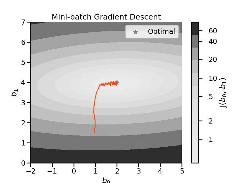
Mini-Batch gradient descent#
Trains on small random subset instead of all data or individual ones.
Performs better than SGD as it exploits hardware optimization of matrix operations
Drawback: It is harder not to end up in local minima
Gradient Descent Comparison#